Discrete Mathematics - More On Graphs

Graph Coloring

Graph coloring is the procedure of assignment of colors to each vertex of a graph G such that no adjacent vertices get same color. The objective is to minimize the number of colors while coloring a graph. The smallest number of colors required to color a graph G is called its chromatic number of that graph. Graph coloring problem is a NP Complete problem.

Method to Color a Graph

The steps required to color a graph G with n number of vertices are as follows −

Step 1 − Arrange the vertices of the graph in some order.

Step 2 − Choose the first vertex and color it with the first color.

Step 3 − Choose the next vertex and color it with the lowest numbered color that has not been colored on any vertices adjacent to it. If all the adjacent vertices are colored with this color, assign a new color to it. Repeat this step until all the vertices are colored.

Example

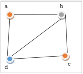
In the above figure, at first vertex a$a$ is colored red. As the adjacent vertices of vertex a are again adjacent, vertex b$b$ and vertex d$d$ are colored with different color, green and blue respectively. Then vertex c$c$ is colored as red as no adjacent vertex of c$c$ is colored red. Hence, we could color the graph by 3 colors. Hence, the chromatic number of the graph is 3.

Applications of Graph Coloring

Some applications of graph coloring include −

• Register Allocation
• Map Coloring
• Bipartite Graph Checking
• Mobile Radio Frequency Assignment
• Making time table, etc.

Graph Traversal

Graph traversal is the problem of visiting all the vertices of a graph in some systematic order. There are mainly two ways to traverse a graph.

• Breadth First Search
• Depth First Search

Breadth First Search

Breadth First Search (BFS) starts at starting level-0 vertex X$X$ of the graph G$G$. Then we visit all the vertices that are the neighbors of X$X$. After visiting, we mark the vertices as "visited," and place them into level-1. Then we start from the level-1 vertices and apply the same method on every level-1 vertex and so on. The BFS traversal terminates when every vertex of the graph has been visited.

BFS Algorithm

The concept is to visit all the neighbor vertices before visiting other neighbor vertices of neighbor vertices.

• Initialize status of all nodes as “Ready”.
• Put source vertex in a queue and change its status to “Waiting”.
• Repeat the following two steps until queue is empty −
  • Remove the first vertex from the queue and mark it as “Visited”.
  • Add to the rear of queue all neighbors of the removed vertex whose status is “Ready”. Mark their status as “Waiting”.

Problem

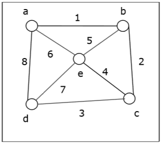
Let us take a graph (Source vertex is ‘a’) and apply the BFS algorithm to find out the traversal order.

Solution −

• Initialize status of all vertices to “Ready”.
• Put a in queue and change its status to “Waiting”.
• Remove a from queue, mark it as “Visited”.
• Add a’s neighbors in “Ready” state b, d and e to end of queue and mark them as “Waiting”.
• Remove b from queue, mark it as “Visited”, put its “Ready” neighbor cat end of queue and mark c as “Waiting”.
• Remove d from queue and mark it as “Visited”. It has no neighbor in “Ready” state.
• Remove e from queue and mark it as “Visited”. It has no neighbor in “Ready” state.
• Remove c from queue and mark it as “Visited”. It has no neighbor in “Ready” state.
• Queue is empty so stop.

So the traversal order is −

a→b→d→e→c$a\to b\to d\to e\to c$

The alternate orders of traversal are −

a→b→e→d→c$a\to b\to e\to d\to c$

Or, a→d→b→e→c$a\to d\to b\to e\to c$

Or, a→e→b→d→c$a\to e\to b\to d\to c$

Or, a→b→e→d→c$a\to b\to e\to d\to c$

Or, a→d→e→b→c$a\to d\to e\to b\to c$

Application of BFS

• Finding the shortest path
• Minimum spanning tree for un-weighted graph
• GPS navigation system
• Detecting cycles in an undirected graph
• Finding all nodes within one connected component

Complexity Analysis

Let G(V,E)$G(V,E)$ be a graph with |V|$|V|$ number of vertices and |E|$|E|$ number of edges. If breadth first search algorithm visits every vertex in the graph and checks every edge, then its time complexity would be −

O(|V|+|E|).O(|E|)$$O(|V|+|E|).O(|E|)$$

It may vary between O(1)$O(1)$ and O(|V2|)$O(|V2|)$

Depth First Search

Depth First Search (DFS) algorithm starts from a vertex v$v$, then it traverses to its adjacent vertex (say x) that has not been visited before and mark as "visited" and goes on with the adjacent vertex of x$x$ and so on.

If at any vertex, it encounters that all the adjacent vertices are visited, then it backtracks until it finds the first vertex having an adjacent vertex that has not been traversed before. Then, it traverses that vertex, continues with its adjacent vertices until it traverses all visited vertices and has to backtrack again. In this way, it will traverse all the vertices reachable from the initial vertex v$v$.

DFS Algorithm

The concept is to visit all the neighbor vertices of a neighbor vertex before visiting the other neighbor vertices.

• Initialize status of all nodes as “Ready”
• Put source vertex in a stack and change its status to “Waiting”
• Repeat the following two steps until stack is empty −
  • Pop the top vertex from the stack and mark it as “Visited”
  • Push onto the top of the stack all neighbors of the removed vertex whose status is “Ready”. Mark their status as “Waiting”.

Problem

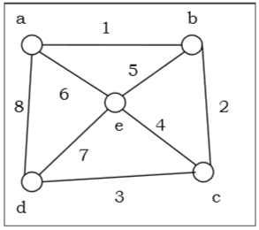
Let us take a graph (Source vertex is ‘a’) and apply the DFS algorithm to find out the traversal order.

Solution

• Initialize status of all vertices to “Ready”.
• Push a in stack and change its status to “Waiting”.
• Pop a and mark it as “Visited”.
• Push a’s neighbors in “Ready” state e, d and b to top of stack and mark them as “Waiting”.
• Pop b from stack, mark it as “Visited”, push its “Ready” neighbor c onto stack.
• Pop c from stack and mark it as “Visited”. It has no “Ready” neighbor.
• Pop d from stack and mark it as “Visited”. It has no “Ready” neighbor.
• Pop e from stack and mark it as “Visited”. It has no “Ready” neighbor.
• Stack is empty. So stop.

So the traversal order is −

a→b→c→d→e$a\to b\to c\to d\to e$

The alternate orders of traversal are −

a→e→b→c→d$a\to e\to b\to c\to d$

Or, a→b→e→c→d$a\to b\to e\to c\to d$

Or, a→d→e→b→c$a\to d\to e\to b\to c$

Or, a→d→c→e→b$a\to d\to c\to e\to b$

Or, a→d→c→b→e$a\to d\to c\to b\to e$

Complexity Analysis

Let G(V,E)$G(V,E)$ be a graph with |V|$|V|$ number of vertices and |E|$|E|$ number of edges. If DFS algorithm visits every vertex in the graph and checks every edge, then the time complexity is −

⊝(|V|+|E|)$$⊝(|V|+|E|)$$

Applications

• Detecting cycle in a graph
• To find topological sorting
• To test if a graph is bipartite
• Finding connected components
• Finding the bridges of a graph
• Finding bi-connectivity in graphs
• Solving the Knight’s Tour problem
• Solving puzzles with only one solution